Reading and print edition
Data Structures Using C
Four sections · Fourteen core chapters · Two appendices
This view includes all lessons. Full executable listings remain in the linked code files; answers are separate so they do not appear beside the questions.
Chapter 01 · Section A
C foundations for data structures
Learning outcomes
Write a small C function, distinguish an array from a structure, and state the contract of a data-structure operation.
1.1 From a problem to a representation
A student-record application stores roll numbers, marks and names. A program must decide both what a value means and how many values are organised. A data type specifies a set of values and permitted operations. A data structure organises values so that operations such as search, insertion and deletion can be performed.
An abstract data type (ADT) describes behaviour without prescribing storage. A stack ADT promises last-in, first-out access. An array and a linked list are two possible implementations. The choice affects capacity, memory use and operation costs, but not the stack's ordering rule.
| Idea | Example | Question answered |
|---|---|---|
| Scalar type | int |
What kind of value is stored? |
| Composite representation | struct Student |
Which fields belong together? |
| Data structure | Array of students | How are many records organised? |
| ADT | Queue | Which operations and ordering rules are available? |
C has arithmetic types, pointers, arrays, structures, unions, enumerations and function types. These language categories should not be confused with the ADT category. C has no built-in class or C++ reference type. In C11, include <stdbool.h> to use bool.
1.2 Control flow and functions
A sequence executes statements in order. Selection chooses a branch with if or switch. Iteration repeats work using for, while or do…while. Choose a loop whose termination condition you can explain.
#include <stddef.h>

/* Contract: a points to n valid int values, or n is zero. */
size_t count_positive(const int a[], size_t n)
{
    size_t count = 0;
    for (size_t i = 0; i < n; ++i) {
        if (a[i] > 0) {
            ++count;
        }
    }
    return count;
}
The counter records how many values satisfy a condition. An accumulator instead combines values, for example a running total. An accumulator's type must have enough range; signed integer overflow is not a valid way to wrap a total in C.
C passes arguments by value. To change a caller's object, pass its address and operate through a pointer. An array parameter such as int a[] is adjusted to a pointer parameter; the function does not receive the array's length automatically.
1.3 Arrays, structures and input
struct Student {
    int roll;
    double mark;
};

struct Student group[3] = {{101, 72.5}, {102, 81.0}, {103, 65.0}};
group[1].mark is the second student's mark. Each structure holds related fields, and the array groups three objects of the same type. Padding may exist between fields, so do not calculate a structure's size by adding field sizes manually.
printf formats output; its conversion specifiers must match the argument types. %d prints an int, %zu prints a size_t, and %f prints a promoted floating-point argument. For input, check the return value of functions such as scanf. For line-oriented input, fgets reads into a bounded buffer; converting and validating the resulting text is a separate step.
1.4 Write the contract before the code
For insertion into an array, a useful contract is: the position is within the logical sequence, spare capacity exists, and success increases the length by one. On failure, the sequence remains unchanged. This prevents a common mistake: writing the happy path without defining full, empty or invalid-input behaviour.
Trace: for {4, -2, 0, 9}, the positive counter after each value is 1, 1, 1, 2. The loop visits four values and uses a fixed amount of extra storage: Θ(n) time and Θ(1) auxiliary space.
Common mistakes
- Treating array length as information a function can infer from a pointer.
- Using an uninitialised variable as a counter or pointer.
- Treating an ADT as inherently static or dynamic. A stack can use either representation.
- Ignoring an input-conversion failure and using an old or uninitialised value.
Practice
- Explain why a queue is an ADT rather than a C language type.
- Trace
count_positivefor{-1, 2, 3, -4, 5}. - Write a function contract for finding the largest element. What should happen for an empty array?
- Design a
struct Bookwith a numeric identifier, a bounded title and a price. Explain one validation rule for each field.
Chapter 02 · Section A
Algorithms and complexity
Learning outcomes
Use stepwise refinement, separate input size from running time, and justify a simple time or space bound.
2.1 Algorithms and invariants
An algorithm is a finite, precisely specified procedure for solving a problem. State its inputs, outputs and preconditions. A useful design sequence is: solve a small example by hand, express the steps, refine each vague step, and test boundary cases.
To find the largest of n values, begin with the first value, compare each remaining value with the current maximum, and replace the maximum when necessary. The precondition is n > 0. The loop invariant is: after processing the first i values, the stored maximum is the largest among those i values. Initialisation, maintenance and termination together explain correctness.
2.2 Count the dominant work
Let n be the number of elements. A full traversal performs n visits. Comparing every unordered pair performs n(n − 1)/2 comparisons. Repeatedly halving a search interval takes a number of steps proportional to log₂ n.
| Growth | Typical pattern | Effect of doubling n |
|---|---|---|
| Θ(1) | Access an array element by index | Essentially unchanged |
| Θ(log n) | Halve a candidate interval | About one additional halving |
| Θ(n) | Visit every element | About twice the work |
| Θ(n log n) | Divide and merge | A little more than twice |
| Θ(n²) | Compare many pairs | About four times |
A bound describes growth, not seconds. Two Θ(n) algorithms may have different constants, cache behaviour or allocation costs. Benchmarking measures a particular implementation and environment; asymptotic analysis explains how cost grows.
2.3 Big O is not the same as worst case
T(n) ∈ O(f(n)) states an asymptotic upper bound: for sufficiently large n, T(n) ≤ c f(n) for some constant c. Ω gives a lower bound and Θ a tight bound. Best, average and worst case describe which inputs of a size are considered. Each case may have its own bound.
For linear search, a successful match in the first position takes Θ(1) time. A missing value requires Θ(n) time. An average-case claim needs an input model; under a uniform distribution of successful positions, the average number of checks is (n + 1)/2.
Writing O(n²) for a linear traversal is technically an upper bound but uninformative. Prefer the tight bound when known. Also state whether “space” means total storage or auxiliary space, the additional workspace beyond the input and output.
2.4 Worked pair-counting example
An inversion is a pair (i, j) for which i < j and a[i] > a[j]. For {8, 4, 2, 1}, the pairs are (8,4), (8,2), (8,1), (4,2), (4,1), (2,1): six inversions.
count = 0
for i = 0 through n − 1:
    for j = i + 1 through n − 1:
        if a[i] > a[j]:
            count = count + 1
return count
The count of comparisons is 3 + 2 + 1 = 6 for n = 4, and n(n − 1)/2 generally. Time is Θ(n²); auxiliary space is Θ(1), assuming a counter wide enough for the result. Equal values are not inversions. A merge-sort-based method can count inversions in Θ(n log n), but it requires a different algorithm and extra workspace.
2.5 Choose a structure by the workload
An array gives constant-time indexed access but may require shifting on insertion. A linked list permits constant-time relinking when the relevant node or predecessor is already known, but finding a position may take linear time. A balanced search tree supports ordered lookup and update in logarithmic time. A hash table targets key lookup rather than sorted traversal.
Ask: which operations dominate, must order be preserved, how large can the collection become, and what memory constraints apply? “Fastest data structure” has no meaning without that workload.
Practice
- How many comparisons are made by the inversion algorithm for n = 6?
- Give the best and worst cases for linear search.
- A loop repeatedly sets
n = n / 2while n is positive. Explain its asymptotic iteration count. - Explain why constant-time insertion into a linked list does not imply constant-time insertion at a numbered position.
Chapter 03 · Section A
Arrays and address calculation
Learning outcomes
Distinguish logical length from capacity, trace insertion and deletion, and calculate one- and two-dimensional array addresses.
3.1 Contiguous elements and valid indices
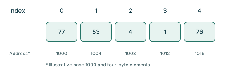
An array is a contiguous sequence of elements of one type. In int a[5], valid indices are 0 through 4. The declaration reserves storage for five integers; it does not imply that an application's sequence currently contains five meaningful records.
Keep capacity and logical length separate. If capacity is 8 and length is 5, operations act on indices 0 through 4 while three slots remain available for insertion. C does not automatically check either boundary.
int a[5] = {23, 12, 7};
Here all five elements exist; the last two are initialised to zero. sizeof a measures the complete local array in bytes. It is 5 * sizeof(int), not necessarily 10 or 20 bytes. An uninitialised automatic array does not receive these zero values.
3.2 Insert without overwriting unread values
Insert 18 at position 2 in {23, 12, 7, 45} with capacity 6.
| Step | Action | Meaningful sequence |
|---|---|---|
| Start | n = 4 | 23, 12, 7, 45 |
| 1 | Copy index 3 to 4 | 23, 12, 7, 45, 45 |
| 2 | Copy index 2 to 3 | 23, 12, 7, 7, 45 |
| 3 | Write 18 at index 2 | 23, 12, 18, 7, 45 |
| 4 | Increase n to 5 | Insertion complete |
Shift right to left so that a source value is not destroyed before it is copied. A valid insertion position satisfies 0 ≤ pos ≤ n. The position n appends. Reject the operation if n == capacity.
if pos < 0 or pos > n or n == capacity: report failure
for i = n down to pos + 1:
    a[i] = a[i − 1]
a[pos] = value
n = n + 1
Deletion requires pos < n. Save the removed value if needed, shift later elements one place to the left, and decrease n. The old final slot may still contain a value, but it is outside the logical sequence. Deleting an element does not shrink the allocated C array.
3.3 Operation costs
| Operation | Time | Reason |
|---|---|---|
| Access by valid index | Θ(1) | Address computed directly |
| Traverse n elements | Θ(n) | Every element visited |
| Insert at end with spare capacity | Θ(1) | One write |
| Insert or delete at the beginning | Θ(n) | Up to n elements shift |
| Search an unsorted array | O(n) worst case | May inspect every element |
A growable array adds an allocation policy. Occasional reallocation is expensive; amortised constant-time append requires a suitable growth strategy and is not a property of a fixed C array.
3.4 Address calculation
For lower bound L, element size w and base address B, the conceptual address is B + (i − L)w. C arrays have lower bound zero. If B = 1000 and w = 4, index 3 has address 1012. These addresses are illustrative, not a promise about an actual program.
For a rectangular array with R rows and C columns in row-major order:
address(A[i][j]) = B + ((i − Lr) × C + (j − Lc)) × w
For int a[3][4], the element a[2][1] is 9 elements from the base. If w = 4 and B = 1000, its illustrative address is 1036. C uses row-major storage for true multidimensional arrays. An array of pointers need not form one contiguous rectangle.
Column-major order instead uses B + ((j − Lc)R + (i − Lr))w. Do not apply the column-major formula to a C rectangular array.
Practice
- Delete position 1 from
{23, 12, 18, 7, 45}. Show every shift. - Explain the difference between
int a[8] = {0};and a logical sequence of length zero. - For a row-major 4 × 5 array, B = 2000 and w = 8, find the address of element
[2][3]. - Test array insertion at the beginning, at the end, into an empty sequence and into a full sequence.
Laboratory: arrays_search.c
Chapter 04 · Section A
Searching techniques
Learning outcomes
Select a search method from its preconditions, trace a binary search interval, and avoid boundary errors.
4.1 Linear search
Linear search inspects elements one at a time until it finds the key or reaches the end. It works whether or not the array is sorted. A useful interface returns a success flag and writes a valid index only on success; this avoids confusing “not found” with index zero.
for i = 0 through n − 1:
    if a[i] == key: return found at i
return not found
For {23, 12, 18, 7, 45} and key 7, the comparisons are 23, 12, 18 and 7. Four elements are inspected. If duplicates exist, this version finds the first occurrence. Best-case time is Θ(1), worst-case time Θ(n), and auxiliary space Θ(1).
4.2 Binary search
Binary search requires an array sorted according to the same ordering used by the search. Inspect the middle value. If the key is smaller, discard the right part; if larger, discard the left part. An arbitrary linked list does not offer the constant-time midpoint access assumed by the array version.
Use a half-open candidate interval [lo, hi): lo is included and hi is excluded. Initially lo = 0 and hi = n. The interval is empty when lo == hi.
lo = 0; hi = n
while lo < hi:
    mid = lo + (hi − lo) / 2
    if a[mid] == key: return found at mid
    if a[mid] < key: lo = mid + 1
    else: hi = mid
return not found
The invariant is: if the key exists and has not been returned, an occurrence remains in [lo, hi). Each unsuccessful step strictly shrinks that interval. Computing the midpoint as lo + (hi − lo)/2 avoids the possible overflow of lo + hi.
4.3 Worked trace
Search for 18 in {7, 12, 18, 23, 45, 60}.
| Step | lo | hi exclusive | mid | Value | Decision |
|---|---|---|---|---|---|
| 1 | 0 | 6 | 3 | 23 | Set hi = 3 |
| 2 | 0 | 3 | 1 | 12 | Set lo = 2 |
| 3 | 2 | 3 | 2 | 18 | Found at index 2 |
For missing key 20, the same first two steps lead to index 2; 18 is too small, so lo becomes 3. Now lo equals hi and the search stops. No access at index 3 is required after the interval becomes empty.
Binary search takes O(log n) worst-case time and Θ(1) auxiliary space in its iterative form. This version may return any matching index when duplicates occur. Finding the first or last occurrence requires a modified boundary search. The laboratory uses such a lower-bound variant: it returns the first matching index, or n when absent. Its return convention differs from the success-flag interface described for linear search above.
4.4 Include preparation in the decision
For one lookup in an unsorted array, sorting first may cost more than linear search. For many searches on mostly unchanged data, an initial sort can be worthwhile. Binary search also does not make insertion into a sorted array logarithmic: finding the position is O(log n), but shifting values may still take Θ(n).
| Situation | Suitable starting choice |
|---|---|
| Small unsorted collection, one query | Linear search |
| Sorted array, repeated queries | Binary search |
| Frequently changing ordered keys | Balanced search tree |
| Key lookup without ordered iteration | Hash table, with collision handling |
Practice
- Trace binary search for 6 and 60 in the six-element array above.
- What happens when n is zero in the half-open algorithm?
- Give an example showing why binary search is invalid on unsorted input.
- Modify the algorithm to return the first index whose value is not less than the key. State how you would then test whether the key exists.
Laboratory: arrays_search.c
Chapter 05 · Section A
Sorting techniques
Learning outcomes
Trace six sorting methods, compare stability and auxiliary space, and explain why pivot and gap choices matter.
5.1 Ordering and stability
Sorting arranges records by a key. Ascending integer order is used here. A stable sort preserves the relative order of records with equal keys. If two students have equal marks, a stable sort by marks preserves their earlier order. Stability is not visible when equal integers carry no distinguishing labels.
An in-place algorithm uses little extra array storage, but recursive calls can still consume stack space. Always state the implementation whose cost is being analysed.
5.2 Bubble, selection and insertion sort
Bubble sort compares adjacent elements and swaps out-of-order pairs. In an ascending pass, the largest remaining value reaches the right end. A swapped flag permits early termination when a whole pass makes no swaps. Use a strict comparison to preserve equal-key order.
Selection sort locates the smallest value in the unsorted suffix and swaps it into the next output position. It performs n(n − 1)/2 key comparisons regardless of initial order. The standard swap-based version is not stable: in {2a, 2b, 1}, swapping 1 with 2a leaves the equal keys ordered 2b, 2a.
Insertion sort maintains a sorted prefix. Save the next key, shift larger prefix values right, and fill the resulting gap. It is useful for small or nearly sorted collections.
| Pass | Key inserted | Array after insertion |
|---|---|---|
| Start | — | 5, 2, 4, 6, 1, 3 |
| 1 | 2 | 2, 5, 4, 6, 1, 3 |
| 2 | 4 | 2, 4, 5, 6, 1, 3 |
| 3 | 6 | 2, 4, 5, 6, 1, 3 |
| 4 | 1 | 1, 2, 4, 5, 6, 3 |
| 5 | 3 | 1, 2, 3, 4, 5, 6 |
Step through insertion sort
An unsigned C index cannot become −1. The lab therefore uses j > 0 and compares a[j − 1] before moving left, rather than decrementing an unsigned j past zero.
5.3 Merge sort
Divide the sequence into two halves, sort each recursively, then merge the sorted halves. During merging, compare the first unconsumed element of each half and copy the smaller one. When one half is exhausted, copy the remainder of the other.
[5,2,4,6] → [5,2] and [4,6]
[5,2] → [5] and [2] → [2,5]
[4,6] → [4] and [6] → [4,6]
merge [2,5] with [4,6] → [2,4,5,6]
Each level processes Θ(n) elements and there are Θ(log n) levels. Standard array merge sort therefore takes Θ(n log n) time. Its temporary array requires Θ(n) storage. Taking from the left half first when keys are equal makes the merge stable.
5.4 Quicksort
Choose a pivot, partition values around it, and recursively sort the two remaining partitions. The supplied lab uses the final element as pivot. For {5, 2, 4, 6, 1, 3}, its first partition produces {2, 1, 3, 6, 5, 4}: pivot 3 reaches index 2. The left and right partitions are not yet internally sorted.
Balanced partitions give Θ(n log n) work. Repeated partitions of sizes zero and n − 1 give Θ(n²). Already sorted input is a bad case for this particular last-pivot implementation. Randomised pivoting improves expected behaviour but does not remove the mathematical quadratic worst case. Standard in-place partitioning is not stable.
5.5 Shell sort
Shell sort performs insertion sorts on elements separated by a gap. Later passes reduce the gap, ending with gap 1. A gap of 3 groups indices (0,3,6,…), (1,4,7,…) and (2,5,8,…). Early movement across long distances can reduce work in the final insertion pass.
for gap = n/2, then gap/2, … while gap > 0:
    for i = gap through n − 1:
        key = a[i]; j = i
        while j >= gap and a[j − gap] > key:
            a[j] = a[j − gap]; j = j − gap
        a[j] = key
There is no single Shell-sort complexity independent of the gap sequence. The simple halving sequence has O(n²) worst-case time. The method uses Θ(1) auxiliary array space and is generally unstable.
5.6 Comparison guide
| Method | Best time | Worst time | Auxiliary space | Stable in described form? |
|---|---|---|---|---|
| Bubble with early exit | Θ(n) | Θ(n²) | Θ(1) | Yes |
| Selection | Θ(n²) | Θ(n²) | Θ(1) | No |
| Insertion | Θ(n) | Θ(n²) | Θ(1) | Yes |
| Merge, standard array | Θ(n log n) | Θ(n log n) | Θ(n) | Yes |
| Quick, last pivot | Θ(n log n) | Θ(n²) | O(n) worst recursion | No |
| Shell, halving gaps | Gap dependent | O(n²) | Θ(1) | No |
Practice
- Trace one bubble pass on
{5, 1, 4, 2}. - Why does insertion sort remain stable when it shifts only values strictly greater than the key?
- Merge
{2, 5, 8}with{1, 5, 9}. Label the two 5s to show stability. - Explain the effect of all-equal input on a two-way last-pivot quicksort. Propose a better partition strategy for many duplicates.
- Compare the number of shifts in insertion sort for sorted and reverse-sorted arrays of length n.
Laboratory: sorting.c
Chapter 06 · Section A
Stacks and queues using arrays
Learning outcomes
Implement bounded stack and queue operations, evaluate a postfix expression, and distinguish circular queues, deques and priority queues.
6.1 Stack operations
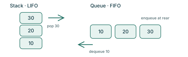
A stack follows last in, first out (LIFO). Push adds an item at the top; pop removes it; peek observes it without removal. With an array and a count size, occupied slots are [0, size). Push writes a[size] then increases size. Pop decreases size then returns a[size].
Check size == capacity before push and size == 0 before pop or peek. A failed operation must not change the stack. Each successful operation takes Θ(1) time in a fixed-capacity array.
6.2 Expressions and the operand order
| Notation | Example |
|---|---|
| Infix | 2 * (4 + 3) - 5 |
| Prefix | - * 2 + 4 3 5 |
| Postfix | 2 4 3 + * 5 - |
To evaluate a binary postfix expression, scan tokens left to right. Push each operand. At an operator, pop the right operand first, then the left; compute left operator right and push the result. Reject an operator with fewer than two operands and reject an expression that ends with anything other than one result. Also validate tokens and arithmetic operations such as division by zero.
| Token | Action | Stack bottom → top |
|---|---|---|
| 2 | Push | 2 |
| 4 | Push | 2, 4 |
| 3 | Push | 2, 4, 3 |
| + | 4 + 3 | 2, 7 |
| * | 2 × 7 | 14 |
| 5 | Push | 14, 5 |
| − | 14 − 5 | 9 |
For infix-to-postfix conversion, output operands immediately. Keep operators on a stack. Before pushing a new operator, pop operators of higher precedence, or equal precedence when the new operator is left-associative. Push (; at ), pop until the matching ( and discard that pair. At the end, pop remaining operators. Mismatched parentheses are errors. Associativity matters for any right-associative operator included in the expression language; C's ^ is bitwise XOR, not exponentiation.
For a mathematical expression language in which ↑ denotes right-associative exponentiation, A ↑ B ↑ C means A ↑ (B ↑ C). Its postfix form is A B C ↑ ↑; popping an equal-precedence ↑ too early would instead impose left association. A unary function such as log consumes one operand, so log(A + B) becomes A B + log. Extend the evaluator's arity checks for such functions; the binary-only algorithm above is not sufficient for them.
Other stack uses include delimiter matching, depth-first search and backtracking. Real source-code delimiter checking must understand strings and comments; counting every bracket character is not a complete parser. To convert 14 to binary, successive remainders are 0, 1, 1, 1; popping them gives 1110. Zero needs its own output case.
6.3 Queue operations
A queue follows first in, first out (FIFO). Enqueue inserts at the rear; dequeue removes from the front. Printer requests, buffers and breadth-first search use this ordering.
A simple non-circular array implementation advances front and rear only to the right. When rear reaches the array end, earlier vacated slots cannot be reused without shifting or resetting. This is a limitation of that implementation, not of the queue ADT.
6.4 Circular queue with an explicit count
Use a strictly positive capacity C, front index f and count n. The next insertion index is (f + n) % C. Enqueue writes there and increments n. Dequeue reads slot f, sets f = (f + 1) % C, and decrements n. Empty means n = 0; full means n = C. All C slots are usable.
| Operation, C = 4 | Physical slots 0,1,2,3 | f | n | Logical queue |
|---|---|---|---|---|
| Enqueue 10,20,30,40 | 10,20,30,40 | 0 | 4 | 10,20,30,40 |
| Dequeue twice | –,–,30,40 | 2 | 2 | 30,40 |
| Enqueue 50 | 50,–,30,40 | 2 | 3 | 30,40,50 |
| Enqueue 60 | 50,60,30,40 | 2 | 4 | 30,40,50,60 |
The dash denotes an unused logical slot; bytes need not be cleared. Never mix these full/empty conditions with a different convention that deliberately leaves one slot unused. Both designs work, but their invariants differ.
6.5 Deques and priority queues
A deque permits insertion and removal at both ends. A circular array can implement all four operations in constant time. An input-restricted deque permits insertion at only one end; an output-restricted deque permits removal at only one end.
A priority queue removes the item with the highest defined priority, not necessarily the earliest arrival. Specify whether a smaller or larger numeric value means higher priority and how equal priorities are handled. A stable policy uses FIFO within equal priorities.
| Representation | Insert | Remove highest priority |
|---|---|---|
| Unsorted array | O(1) with room | O(n) search |
| Sorted array | O(n) shifts | O(1) from chosen end |
| Binary heap | O(log n) | O(log n) |
These are implementation costs, not universal costs for the ADT. A binary heap supports O(1) inspection of the extreme key at its root.
Practice
- Evaluate postfix
8 3 - 2 *and explain why operand order matters. - A capacity-four ring has front 3 and count 2. Which slots are occupied and where is the next enqueue?
- Compare a deque with a priority queue using one application for each.
- Design tests for full-to-nonfull and one-element-to-empty transitions.
- Convert
(A + B) * C - Dto postfix.
Laboratory: stack_queue.c
Chapter 07 · Section B
Pointers and dynamic memory
Learning outcomes
Read pointer expressions, allocate a node safely, and explain ownership, lifetime and cleanup.
7.1 Addresses and indirection
A pointer stores an address used to access an object or function. With int x = 7; int *p = &x;, p points to x and *p accesses x. The expression *p = 9 changes x. Declaring a pointer does not create the object it should point to.
A null pointer indicates the absence of a target; do not dereference it. A dangling pointer refers to an object whose lifetime has ended. A pointer may also be non-null and still invalid. A null check alone does not prove validity.
7.2 Arrays and pointer arithmetic
For an array a, the expression a[i] is equivalent to *(a + i). Pointer arithmetic advances by elements of the pointed-to type, not raw bytes. A pointer one past the end may be formed for comparison or iteration, but must not be dereferenced. Arithmetic and relational comparisons must respect the C rules for the underlying array object.
int a[3] = {10, 20, 30};
int *p = a;
/* *(p + 1) is 20. */
int *rows[3] is an array of three pointers. int (*p)[3] is a pointer to an array of three integers. Parentheses change the declaration. The first form alone does not allocate any row data.
7.3 Structures and nodes
struct Node {
    int value;
    struct Node *next;
};
A node stores one value and a link. node->value is shorthand for (*node).value. A structure cannot contain an ordinary instance of itself, which would require unbounded size, but it can contain a pointer to its own type.
7.4 Dynamic allocation
malloc allocates a requested number of bytes and returns a pointer, or a null pointer on failure. calloc also sets allocated bytes to zero. Do not generalise byte-zeroing to every possible pointer or floating representation; initialise fields according to their types. free ends the lifetime of a previously allocated block. Free each owned block once, and do not access it afterwards.
#include <stdlib.h>

struct Node *node = malloc(sizeof *node);
if (node == NULL) {
    /* Report allocation failure; leave the structure unchanged. */
} else {
    node->value = 25;
    node->next = NULL;
    /* Transfer ownership to a list, or free(node) when finished. */
}
In C, no cast is needed for the result of malloc. Include <stdlib.h> so the compiler has its declaration. sizeof *node follows the pointed-to type automatically. When allocating n elements, check that n * sizeof *p will not overflow size_t before calling the allocator.
If using realloc with a nonzero new size, assign its result to a temporary pointer. On failure the original allocation remains valid; assigning directly to the only owning pointer can lose the address and leak the block.
7.5 Ownership and failure paths
A list's head owns the chain in these examples. A search result is a borrowed pointer: it may observe a node but does not own an additional allocation. Removing the node invalidates that borrowed pointer.
To delete the first node: save its address, move head to the next node, then free the saved node. Reversing the last two actions would read a freed object. For complete cleanup, repeat until head is null. Setting one pointer to null after free does not repair other aliases to the same freed object.
A sound allocation policy is transactional at the operation level: allocate first; only after success link the new object into the structure. If allocation fails, return an error without changing the existing links.
Practice
- Explain the difference between a null pointer and a dangling pointer.
- Why is
sizeof pnormally wrong when allocating storage for an object of the type pointed to by p? - Trace the safe deletion of the head of a two-node list.
- Explain why calling
freeon the same block twice is invalid even if two pointer variables hold its address.
Laboratory: linked_list.c
Chapter 08 · Section B
Linked lists
Learning outcomes
Trace insertion, deletion and reversal in a singly linked list, compare list variants, and account for search cost.
8.1 Links rather than consecutive positions
A linked list connects nodes through stored addresses. Nodes need not be adjacent in memory. A head pointer identifies the first node; a null head represents an empty singly linked list. The last node's next link is null.
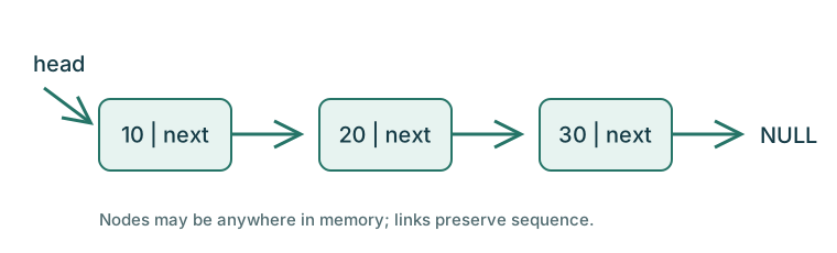
Lists can grow node by node, but each node carries pointer and allocation overhead. Arrays usually offer better locality and constant-time indexed access. “Dynamic” does not mean that insertion can never fail: allocation can fail.
8.2 Insert at the beginning or after a node
To prepend value x, allocate a new node, set its value, point its next field to the old head, and then make head point to it. This works unchanged for an empty list.
new.next = head
head = new
To insert after a known node p, first set new.next = p.next, then set p.next = new. Reversing those assignments can lose the remainder of the list. Relinking is Θ(1); finding p may be Θ(n).
Appending is Θ(n) if only head is retained and traversal is needed to find the last node. With a valid tail pointer, append is Θ(1), but every operation that empties or changes the last node must maintain tail.
8.3 Remove the first matching value
Search while retaining the current node and its predecessor. If no match exists, return failure without changing the list. If the matching node is head, advance head. Otherwise, set previous.next = current.next. Save any required value, free the removed node and do not use its pointer again.
| Delete 20 from 10 → 20 → 30 | State |
|---|---|
| Locate | previous = node 10; current = node 20 |
| Bypass | node 10 next becomes node 30 |
| Release | Free node 20 |
| Result | 10 → 30 → NULL |
Deletion by key is O(n) because of the search. Deletion after a known predecessor is Θ(1). In a singly linked list, an arbitrary pointer to a node does not generally provide its predecessor.
8.4 Reverse the links
previous = NULL
current = head
while current != NULL:
    following = current.next
    current.next = previous
    previous = current
    current = following
head = previous
Saving following before reversing the link preserves access to the unprocessed suffix. At every step, previous heads the reversed prefix and current heads the unreversed suffix. Time is Θ(n), auxiliary space Θ(1). Empty and singleton lists need no special branch.
8.5 Variants
| Variant | Representation | Benefit | Extra care |
|---|---|---|---|
| Doubly linked | Each node has prev and next | Bidirectional traversal; unlink known node | Update both directions and endpoints |
| Circular singly linked | Last next points to first | Repeated round-robin traversal | Stop on return to start, not on NULL |
| Header or sentinel list | Extra non-data node anchors links | Fewer boundary special cases | Do not treat sentinel as user data |
For a doubly linked insertion between p and q, connect the new node to both neighbours, then update p.next and q.prev. If either neighbour is absent, update the corresponding endpoint. A circular list with a tail pointer can reach its first node as tail->next when nonempty; deleting its sole node must also reset tail.
A polynomial may be represented as a list of (coefficient, exponent) terms ordered by exponent. Merging two such lists supports addition by combining equal exponents. Eliminate zero-coefficient terms if that is part of the representation invariant.
Practice
- Prepend 5 to the list in Figure 8.1. Show which links change.
- Trace reversal of 10 → 20 → 30, recording previous, current and following.
- State the invariant for an empty and a singleton circular list using tail.
- Why does a doubly linked list need more writes during insertion than a singly linked list?
- Design a polynomial-addition procedure for two exponent-sorted term lists.
Laboratory: linked_list.c
Chapter 09 · Section B
Linked stacks and queues
Learning outcomes
Use linked-list operations to implement stack and queue ADTs, and preserve endpoint invariants through empty transitions.
9.1 Linked stack
Let top point to the first node. Push is insertion at the head; pop is deletion at the head. Both perform a constant number of pointer updates. A push also requires allocation, which can fail. “No fixed capacity” is not the same as unlimited memory.
PUSH(x):
    allocate new node; if allocation fails, report failure
    new.value = x
    new.next = top
    top = new

POP():
    if top is NULL: report underflow
    old = top
    result = old.value
    top = old.next
    free old
    return result
After pushing 10, 20 and 30, top points to 30 → 20 → 10 → NULL. Popping returns 30 and leaves 20 → 10 → NULL. The operation must save the returned value before freeing its node.
The pointer-update cost is Θ(1); the cost of the system allocator is normally abstracted away in this introductory analysis. Displaying all elements is Θ(n), and total node storage is Θ(n). If constant-time size is required, maintain a count rather than traversing for every size query.
9.2 Linked queue
A queue retains two endpoints: front points to the next item to remove, and rear points to the last node. Enqueue at rear and dequeue at front.
Invariant: an empty queue has both front and rear null. A nonempty queue has a reachable rear node whose next link is null.
ENQUEUE(x):
    allocate new node; if allocation fails, report failure
    new.value = x; new.next = NULL
    if rear is NULL: front = new
    else: rear.next = new
    rear = new

DEQUEUE():
    if front is NULL: report underflow
    old = front; result = old.value
    front = old.next
    if front is NULL: rear = NULL
    free old
    return result
The reset of rear is essential. Without it, removing the final node leaves a dangling rear pointer, and a later enqueue may write through freed storage.
9.3 Worked boundary trace
| Operation | Front | Rear | Sequence |
|---|---|---|---|
| Start | NULL | NULL | Empty |
| Enqueue 10 | node 10 | node 10 | 10 |
| Enqueue 20 | node 10 | node 20 | 10, 20 |
| Dequeue | node 20 | node 20 | 20 |
| Dequeue | NULL | NULL | Empty |
| Enqueue 30 | node 30 | node 30 | 30 |
Each enqueue or dequeue performs Θ(1) link work. No shifting or modular arithmetic is needed, but node links and allocations add overhead. For a bounded buffer with predictable memory use, a circular array may be the better choice.
9.4 Design the API around failure
Returning a special integer such as −1 is ambiguous if −1 is valid data. A boolean success result plus an output pointer separates status from value. The output remains unchanged on failure. Document pointer validity as a precondition and define who owns each allocated node.
Test an empty pop, a full lifecycle from empty to populated and back, repeated reuse after emptying, and cleanup with remaining elements. Allocation-failure testing requires a controllable allocator or fault-injection wrapper; ordinary successful runs do not prove that path was executed.
Practice
- Show the linked stack after pushing 7, pushing 9, popping, and pushing 4.
- Explain why a linked queue with only a front pointer cannot generally enqueue in Θ(1) time.
- Identify the unsafe statement if code frees old before evaluating
old->next. - Write a queue cleanup algorithm and state its final endpoint invariant.
Laboratory: linked_stack_queue.c
Chapter 10 · Section C
Trees and binary search trees
Learning outcomes
Classify binary trees, trace recursive and iterative traversals, and explain how BST shape controls performance.
10.1 Tree vocabulary
A tree is a connected acyclic structure. In a rooted tree, each non-root node has one parent; nodes may have children. A leaf has no children. The depth of a node is the number of edges from the root. In this book, the height of a nonempty tree is the maximum number of edges from its root to a leaf; a leaf has height zero. Implementations may store node-count heights instead, provided their formulas remain consistent.
A binary tree gives each node at most a left and a right child. Full means every node has zero or two children. Complete means all levels except possibly the last are full, and the last fills left to right. Perfect means every internal node has two children and all leaves have the same depth. A skewed tree can have height n − 1.
10.2 Representation
A linked node contains a key, a left pointer and a right pointer. A zero-based array representation places the children of index i at 2i + 1 and 2i + 2, if those positions exist. The parent of a non-root index i is (i − 1)/2 using integer division. This is efficient for complete trees such as binary heaps, but sparse shapes can waste array positions.
10.3 Traversal orders
| Traversal | Rule | Result for Figure 10.1 |
|---|---|---|
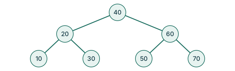
| Preorder | Node, left, right | 40, 20, 10, 30, 60, 50, 70 |
| Inorder | Left, node, right | 10, 20, 30, 40, 50, 60, 70 |
| Postorder | Left, right, node | 10, 30, 20, 50, 70, 60, 40 |
| Level order | Increasing depth, left to right | 40, 20, 60, 10, 30, 50, 70 |
In recursive traversal, return immediately for a null pointer. Each real node is visited once, so time is Θ(n). Auxiliary call-stack space is O(h + 1), where h is the edge-count height of a nonempty tree. This includes the one-frame requirement for a leaf with h = 0. It can be O(n) for a skewed tree. Level-order traversal uses a queue whose size is proportional to the maximum width.
For iterative inorder, keep a stack and current pointer. Push current and move left until null; pop a node and visit it; then set current to its right child. Repeat while current is non-null or the stack is nonempty. The explicit stack preserves the same pending work as recursion.
10.4 Binary search tree operations
A BST maintains an ordering rule: all keys in a node's left subtree are smaller, and all keys in its right subtree are larger. The labs ignore duplicate keys. Other policies are possible, such as storing a frequency, but must be stated explicitly.
Search compares the requested key with the current key and descends into only one child. Insertion follows that path until it reaches an empty link, where it attaches a new node. Inorder traversal yields sorted keys because of the BST invariant, not merely because the tree is binary.
Deletion has three cases:
- Leaf: remove its link from the parent.
- One child: replace the node's link with its child.
- Two children: copy the inorder successor's key (the minimum in the right subtree), then delete that successor from its original position. The successor has no left child.
If nodes store records rather than isolated keys, copy or transfer the associated payload consistently. If deleting the root, update the root pointer. Release each removed allocation exactly once.
10.5 Shape and complexity
Search, insertion and deletion follow paths of length O(h). Balanced height gives O(log n); a skewed BST gives O(n). Inserting sorted keys into an ordinary BST can produce a chain. A tree does not become balanced merely because it is a binary search tree.
A binary heap instead maintains a parent–child priority relation and a complete shape. It does not enforce the full BST ordering rule. A heap is suitable for priority queues; a BST is suitable for ordered search. AVL trees enforce balance explicitly in Chapter 14.
Practice
- Write the preorder, inorder and postorder for root 8 with left child 3 and right child 10, where 3 has right child 6.
- Insert 10, 20, 30 and 40 into an ordinary BST. What is its height?
- Delete root 40 from Figure 10.1 using its inorder successor.
- Explain why postorder is a natural order for freeing every node of a linked tree.
- Give a tree that is full but not complete.
Laboratory: bst.c
Chapter 11 · Section C
Threaded trees and B-trees
Learning outcomes
Explain the purpose of threads, state B-tree occupancy rules under a declared convention, and trace a split.
11.1 Threaded binary trees
In an ordinary linked binary tree, many child pointers are null. A threaded tree uses selected otherwise-null pointers to store traversal links, commonly inorder predecessors or successors. Tag fields distinguish a real child from a thread. Treating a thread as a child can create an infinite traversal.
In a right-threaded tree, a node with no right child may point to its inorder successor. To find the successor of node p: follow the right thread if one exists; otherwise enter p's real right subtree and repeatedly follow real left children to its leftmost node. A header sentinel can represent traversal boundaries.
For a BST with keys 10, 20 and 30 and root 20, node 10's missing right child can thread to 20. An inorder traversal visits 10, follows that thread to 20, then visits 30 through the real right subtree. Insertion and deletion must preserve both ordinary child links and thread links. Threads trade update complexity for traversal without a separate recursion stack.
11.2 Why multiway trees are useful
A binary tree makes one left/right decision at each node. A multiway search tree stores several sorted keys in a node, dividing the key range into several child intervals. When nodes correspond to storage pages, greater branching can reduce the number of page visits. CPU comparisons within a node and storage accesses are distinct costs.
A B-tree maintains bounded occupancy and places every leaf at the same depth. This chapter uses minimum degree t, with t ≥ 2, to avoid ambiguity in the word “order”.
| Property | Rule |
|---|---|
| Maximum keys in any node | 2t − 1 |
| Minimum keys in a non-root node | t − 1 |
| Children of an internal node with k keys | k + 1 |
| Maximum children | 2t |
| Nonempty root | At least one key |
| Internal root | At least two children |
| Leaf depth | Same for all leaves |
An empty tree may use an empty root or a null root, depending on the implementation. Some texts define order m as maximum children; always confirm that convention before translating a question.
11.3 Search and a split trace
For keys [20, 40], the child ranges are values below 20, values between 20 and 40, and values above 40, under a no-duplicates policy. Search first checks the keys in the node; if absent, it descends into the appropriate range.
Take t = 2, so each node holds at most three keys. Insert 10, 20 and 30: the root becomes [10,20,30]. Before descending to insert 40, split the full root. Promote 20 to a new root, with leaf children [10] and [30]. Insert 40 into the right leaf, giving [30,40].
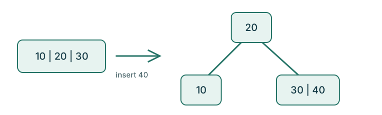
The promoted key belongs to the parent, not both leaves, in this B-tree convention. A B+ tree follows different leaf-storage rules and should not be treated as identical.
11.4 Deletion at concept level
Deletion must preserve minimum occupancy. If a target key is in an internal node, use a suitable predecessor or successor when the corresponding child can spare a key. Otherwise, combine the neighbouring children and separating parent key, then continue. Before descending into a minimally occupied child, borrow through the parent from a sibling with spare keys or merge with a sibling. An empty internal root can be replaced by its only child, decreasing height.
For fixed t, height is O(log n), giving logarithmic search and update paths. The detailed cost also depends on work within each node. This chapter develops the invariants and split reasoning; a production B-tree implementation additionally needs tested merge, borrow, root-change and storage-management paths.
Practice
- Why must a threaded-tree pointer carry a child/thread tag?
- For t = 3, state the minimum and maximum keys in a non-root node.
- Continue the t = 2 insertion example with 50 and 60. Show any split.
- Explain why a B-tree root may have fewer keys than a non-root node.
Chapter 12 · Section C
Graphs and traversal
Learning outcomes
Choose a graph representation, trace BFS and DFS, and distinguish shortest paths from minimum spanning trees.
12.1 Vertices, edges and representations
A graph G = (V, E) consists of vertices and edges. Directed edges have an orientation; undirected edges connect unordered pairs. A weighted graph associates costs with edges. A path follows edges, a cycle returns to its starting vertex, and connected components identify mutually reachable groups in an undirected graph.
| Representation | Storage | Check one edge | Enumerate neighbours |
|---|---|---|---|
| Adjacency matrix | Θ(V²) | Θ(1) | Θ(V) |
| Adjacency lists | Θ(V + E) | O(degree) in unsorted list | Θ(degree) |
| Edge set/list | Θ(V + E) including vertices | O(E) by linear scan | O(E) by scan |
For an undirected adjacency list, each edge is usually recorded twice. A matrix for an undirected graph is symmetric. A weighted representation must distinguish a missing edge from a zero-weight edge; using zero for both loses information. A graph's vertex set also includes isolated vertices, which do not appear in any edge pair.
12.2 Breadth-first search
BFS explores vertices in distance layers from a start vertex. Mark the start discovered and enqueue it. Repeatedly dequeue a vertex, examine its neighbours, and mark and enqueue each undiscovered neighbour. Mark when enqueuing, not later, to prevent repeated queue entries.
Use edges {0–1, 0–2, 1–3, 2–3, 2–4} and inspect neighbours in increasing numeric order.
| Removed vertex | Newly discovered | Queue afterwards |
|---|---|---|
| Start | 0 | 0 |
| 0 | 1, 2 | 1, 2 |
| 1 | 3 | 2, 3 |
| 2 | 4 | 3, 4 |
| 3 | None | 4 |
| 4 | None | Empty |
Visit order is 0, 1, 2, 3, 4. BFS distances from 0 are 0, 1, 1, 2, 2. Store a predecessor when discovering each vertex to reconstruct a shortest path in an unweighted graph.
12.3 Depth-first search
DFS visits a vertex, marks it and recursively visits each undiscovered neighbour, completing one branch before returning. For the same graph and neighbour order, the lab produces 0, 1, 3, 2, 4. An explicit stack can replace recursion, though push order affects the resulting traversal order.
With adjacency lists, both BFS and DFS take Θ(V + E) for a full traversal. The lab also includes a self-loop at 2 and isolated vertex 5 as boundary tests; neither changes the stated traversal orders from 0. The supplied matrix lab scans a full row for each visited vertex, so its worst-case time is Θ(V²). Both need O(V) traversal state. To cover a disconnected graph, start another traversal at each still-undiscovered vertex; one starting vertex covers only its reachable component.
12.4 Dijkstra's shortest paths
Dijkstra's algorithm computes shortest-path distances from one source when edge weights are nonnegative. Initialise the source to zero and other distances to infinity. Repeatedly settle the unsettled vertex with smallest tentative distance, then relax its outgoing edges: replace a neighbour's distance if the path through the settled vertex is shorter. Stop if no reachable unsettled vertex remains.
For undirected edges A–B:4, A–C:1, C–B:2, B–D:1, C–D:5, D–E:3, B–E:7, the final distances from A are:
| Vertex | Distance | Path |
|---|---|---|
| A | 0 | A |
| C | 1 | A → C |
| B | 3 | A → C → B |
| D | 4 | A → C → B → D |
| E | 7 | A → C → B → D → E |
An array-based minimum selection gives O(V²) time. Adjacency lists with a suitable binary heap give O((V + E) log V). Negative edges invalidate the settling argument; use an algorithm whose assumptions permit them. Unreachable vertices remain at infinity, and code must avoid overflowing a distance when adding weights.
12.5 Minimum spanning trees
A spanning tree connects all vertices of a connected undirected graph without a cycle. It has V − 1 edges. An MST minimises total tree weight, not distance from one source.
Prim's algorithm grows one tree, repeatedly choosing a minimum-weight edge crossing from the selected vertices to an unselected vertex. Kruskal's algorithm processes edges in nondecreasing weight order and accepts an edge only when it joins different components, usually tracked by disjoint-set union.
For the complete graph on {1,2,3,4,5} with w(i,j) = |i − j|, the edges 1–2, 2–3, 3–4, 4–5 form a tree of total weight 4. Every spanning tree has four edges and every edge weighs at least 1, so no smaller total is possible. This supplies a lower-bound argument as well as a construction.
For a disconnected graph, the corresponding result is a minimum spanning forest. Equal weights may permit several MSTs. The choice between Prim and Kruskal depends on representation and implementation, not solely on the label “sparse” or “dense”.
Practice
- Add isolated vertex 5 to the traversal example. Does BFS from 0 visit it?
- Build the adjacency matrix for the five-vertex traversal graph.
- Explain why BFS is not generally a weighted shortest-path algorithm.
- Give a reason that a shortest-path tree and an MST can differ.
- State what Kruskal's component test prevents.
Laboratory: graph_traversal.c
Chapter 13 · Section D
File handling in C
Learning outcomes
Distinguish file organisation from in-memory representation, use streams safely, and explain the portability limits of raw structure storage.
13.1 Data, information and persistence
Data are recorded values; information is the meaning obtained by interpreting them in context. A mark of 75 becomes useful when associated with a student, assessment and scale. A data structure organises values during execution. A file preserves encoded data beyond the lifetime of the process.
A file format defines how values are represented. File organisation defines how records are arranged and accessed. Sequential organisation reads records in order; indexed organisation adds a structure for locating records by a key; direct or hashed organisation maps keys to locations under a defined policy. These are design choices, not alternative names for C file-opening modes.
13.2 Streams and modes
C's standard I/O library uses a FILE * to manage a stream. Open with fopen, check for failure, perform checked operations and close with fclose. Closing may itself report a write failure, so do not assume that a previous successful write guarantees durable output.
| Mode | Meaning | Important consequence |
|---|---|---|
r |
Read existing file | Fails if it cannot be opened |
w |
Write | Creates or truncates a file |
a |
Append | Writes go to the end |
r+ |
Read and write existing file | Does not truncate on open |
wb / rb |
Binary write/read | Binary mode where relevant |
Use a temporary test file rather than an important existing file during experiments. The provided lab uses tmpfile, which creates a temporary stream for update and avoids choosing an external filename.
13.3 Text records
A text format might store roll mark on each line, for example 101 72.50. fprintf writes formatted text. Read bounded lines with fgets and parse them when records require robust validation. For a controlled numeric demonstration, fscanf is acceptable if the program checks how many conversions succeeded and handles malformed input.
open stream; if failure, report error
for each record:
    write fields; if failure, close and report error
flush and reposition if switching to reading
read records while the required conversions succeed
distinguish end of file from malformed data and I/O failure
close stream and check status
Do not use while (!feof(file)) as the read loop. End-of-file status becomes set after an attempted read encounters the end; it does not predict whether the next record can be read. Drive the loop with the read operation's result.
Update streams have sequencing rules when alternating reads and writes. A positioning operation such as fseek is a simple way to establish the intended position and direction after writing. Check its return value; not every stream is seekable.
13.4 Binary records and portability
fread and fwrite transfer objects as bytes and report the number of complete items transferred. Writing a whole structure with fwrite may be convenient for a local experiment, but it is not a portable interchange format: padding, integer sizes, byte order and floating representation can vary. A stored pointer is not a useful link when the file is loaded into another process.
A durable format should define field widths, encoding, byte order, record boundaries and versioning. Validate lengths and offsets before allocating or accessing memory. Fixed-size records can support calculated offsets, but the file format—not an assumed compiler layout—must define their size.
13.5 Connect files to data structures
A student-record system can load records into a list for editing, sort an array of records for reporting and build an index for repeated lookup. Saving the result is a distinct operation. If reliability matters, replacing a file safely may require a temporary output, checked flush/close operations and a platform-specific replacement policy; a simple fopen("records.txt", "w") truncates immediately.
The laboratory demonstrates the smaller, reproducible task: write two student records (roll number, one-word name and mark) to a temporary stream, reposition, read them back and assert equality. It does not implement a general database, recovery scheme or persistent index.
Practice
- Why can opening a file with
wdestroy information before the first explicit write? - Explain the error in
while (!feof(fp)) { fscanf(...); process(record); }. - Why should a linked-list node's raw pointer not be stored as a persistent link?
- Propose a simple text format for student records and identify two malformed-record cases.
Laboratory: file_records.c
Chapter 14 · Section D
AVL trees, sets and skip lists
Learning outcomes
Identify AVL imbalance cases, perform basic set operations and explain the probabilistic structure of a skip list.
14.1 AVL balance
An AVL tree is a BST in which every node's left and right subtree heights differ by at most one. Define the balance factor as height(left) − height(right). Allowed values are −1, 0 and +1. The lab stores null height 0 and leaf height 1; this differs by a constant from edge-count height, but balance factors are unchanged.
After insertion, update heights on the path to the root. At the first unbalanced ancestor, identify the heavy path and rotate while preserving inorder key order.
| Heavy path | Common name | Repair |
|---|---|---|
| Left then left | LL | Right rotation |
| Right then right | RR | Left rotation |
| Left then right | LR | Left rotation on child, then right on ancestor |
| Right then left | RL | Right rotation on child, then left on ancestor |
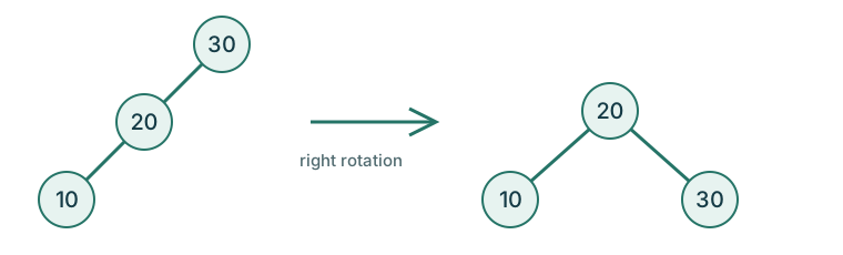
For insertion 30, 20, 10, node 30 becomes left-heavy by two; a right rotation makes 20 the root. For 30, 10, 20, first rotate left at 10, then right at 30. Do not select a rotation by looking only at the imbalance sign; the child's shape matters too.
The laboratory inserts 30, 100, 150, 20, 10, 45, 80, 75, 120, 130, 125, 200, 75, ignoring the duplicate 75. Its final inorder sequence is 10, 20, 30, 45, 75, 80, 100, 120, 125, 130, 150, 200. Checking sorted order alone is insufficient: tests must also verify every stored height and every balance factor after each update.
14.2 AVL deletion reasoning
Delete as in a BST, then update heights and rebalance while returning towards the root. Unlike insertion, deletion can require repairs at multiple ancestors. The child balance factor may be zero, so insertion-key comparisons are not a valid deletion rotation rule.
Consider keys 100, 50, 150, 25, 75, 125, 175, 10, 30, 60. Deleting 75 replaces that one-child node with 60. At node 50, the left subtree rooted at 25 has edge-height 1 and the right leaf 60 has height 0; its balance factor is +1. The root remains balanced, so no rotation is required. An update is not obliged to rotate merely because the structure is an AVL tree.
AVL search, insertion and deletion take O(log n) worst-case time when the balance invariant is maintained. The supplied executable implements insertion; deletion above is a reasoning exercise, not a claim that the lab implements it.
14.3 Sets and list representation
A set contains distinct elements. Membership asks whether a value is present. Union contains elements in either set; intersection contains elements in both; difference A − B contains elements in A but not B.
For A = {1,3,5} and B = {3,4,5}, union is {1,3,4,5}, intersection {3,5}, and A − B is {1}. Difference is not commutative.
An unsorted list implements membership in O(n). Inserting a value while preserving uniqueness needs a membership test unless a stronger precondition is provided. For two sorted distinct-element lists of lengths m and n, two-pointer merging computes union or intersection in O(m + n) time, using output space proportional to the result.
Applications include removing duplicate identifiers, tracking visited graph vertices and comparing access lists. The appropriate representation depends on key range and workload: bit sets suit bounded integer universes, hash sets suit membership, and balanced trees also support ordered iteration.
14.4 Skip lists
A skip list has a sorted base-level list and additional forward links that skip over groups of elements. Random promotion gives some nodes taller “towers”. To search, begin at the highest level, move right while the next key is less than the target, then move down. At the base level, check the next key for equality.
Insertion records the predecessor at each visited level, chooses the new node's height and reconnects the relevant forward links. Deletion bypasses the target on every level where it occurs. Under a standard independent geometric-height model, search, insertion and deletion have expected O(log n) time and expected O(n) total link storage. A poor random outcome can still produce O(n) search time; this is an expected bound, not AVL-style deterministic balance. OpenDSA's skip-list explanation develops this distinction.
Level 2: HEAD ───────────────→ 20 ───────────────→ END
Level 1: HEAD ───→ 10 ──────→ 20 ──────→ 40 ───→ END
Level 0: HEAD → 5 → 10 → 15 → 20 → 30 → 40 → 50 → END
To search for 30, reach 20 on the upper level, descend when the next jump would overshoot, and then follow the base-level link to 30. The diagram is an example tower arrangement, not a uniquely determined structure for these keys.
Practice
- Which rotation repairs insertion of 10, 30, 20 into an empty AVL tree?
- Why does AVL deletion need to continue checking ancestors after one repair?
- Compute union, intersection and both differences for
{2,4,6}and{1,4,7}. - Contrast the worst-case guarantee of AVL search with the expected bound of skip-list search.
- Explain how a sorted-list intersection advances pointers when the two current values differ.
Laboratory: avl.c
Appendix A · Enrichment
Hashing
Learning outcomes
Resolve collisions, calculate load factor and explain why open-address deletion needs a special marker.
A.1 Key-to-slot mapping
Hashing maps a key to a table position using a hash function. A collision occurs when different keys map to the same slot. Collisions are normal; a correct table must handle them. Load factor is number of stored keys / number of slots.
A hash table is not a sorted structure. Expected constant-time lookup depends on assumptions about hashing, load and collision handling; worst-case lookup can be linear.
A.2 Chaining and open addressing
Chaining stores a collection of keys at each bucket. Open addressing stores keys in table slots and probes alternatives after a collision. Linear probing uses consecutive slots with wraparound; quadratic probing and double hashing use different probe sequences and require suitable table-size and step choices.
For capacity 7 and h(k) = k mod 7 on nonnegative keys, 10, 17 and 24 all start at slot 3. Linear probing places them at 3, 4 and 5. Searching for 24 must inspect the intervening occupied slots.
A.3 Deletion and tombstones
If 17 is removed and slot 4 is simply marked never-used, a search may stop there and incorrectly report 24 absent. Mark it deleted, or tombstone, instead. Lookup continues through a tombstone but may stop at a never-used slot. Insertion may reuse a tombstone after checking that the key is not already present later in the probe sequence.
Bound every probe by table capacity. A full table or one containing only tombstones must not cause an infinite loop. The supplied integer-set lab uses capacity 7, distinguishes empty/occupied/deleted states and rejects a new key when no slot is available. It does not resize.
Practice
- Insert 8, 15 and 22 into an empty capacity-seven linear-probing table.
- Why is a tombstone different from an unused slot?
- Explain why a hash table does not directly answer “print keys in sorted order”.
Laboratory: hashing.c
Appendix B · Enrichment
C++ comparison
Purpose
The main chapters and laboratories use C11. This appendix shows the same pair-counting idea in C++17 so that C++ examination material can be read without mixing language syntax into the C implementations.
B.1 The algorithm stays the same
An inversion has i < j and a[i] > a[j]. The following C++ program stores four values in std::array, compares every pair, checks the answer and prints it.
#include <array>
#include <cassert>
#include <cstddef>
#include <iostream>

int main()
{
    const std::array<int, 4> a{8, 4, 2, 1};
    std::size_t inversions = 0;
    for (std::size_t i = 0; i < a.size(); ++i) {
        for (std::size_t j = i + 1; j < a.size(); ++j) {
            if (a[i] > a[j]) {
                ++inversions;
            }
        }
    }
    assert(inversions == 6);
    std::cout << "Inversions: " << inversions << '\n';
}
Time is Θ(n²), with Θ(1) extra scalar workspace for this pair-counting method. For large n, the chosen count type must hold up to n(n − 1)/2. The fixed four-element demonstration has no overflow risk.
B.2 Keep the language boundaries explicit
| C11 | C++17 |
|---|---|
printf from <stdio.h> |
Stream output with std::cout from <iostream> |
struct Node * unless a typedef exists |
A declared structure name may be used directly as a type |
malloc / free for raw allocated storage |
Constructors/destructors and RAII support managed object lifetimes |
| No C++ reference types or classes | References and classes are language features |
Do not mix malloc with delete, or new with free. Prefer ownership-aware C++ containers and resource management rather than copying a C allocation pattern mechanically. The ADT invariants—LIFO, FIFO, BST ordering—remain meaningful in both languages.
Practice
- Change the array to
{1, 3, 2, 4}and predict the inversion count before running it. - Why does changing
>to>=alter the definition when duplicate values occur?
Laboratory: inversions.cpp